Clock And Timestamp
1 Preface
这篇文章总结了几个分布式数据库系统中常用的时钟算法, 主要包括: 中心授时服务, Google True Time, NTP, Logical clock, HLC.
花了比较大篇幅描述HLC的算法实现以及它的优缺点.
2 Why do we need clock/timestamp in (distributed) DBMS?
为什么需要时钟 -> 因为需要mvcc -> 为什么需要mvcc -> 因为事务需要锁, 需要解决事务冲突冲突
为什么不能使用本地时间? 如果使用本地时间, 没法保证内部系统的数据一致性(由于时间不统一, 节点1写入数据在 节点2可能读不到).
3 Terminology
| item | meaning | note |
|---|---|---|
hb |
happened-before | |
⇒ |
implies | |
∧ |
logical AND | |
e ∥ f |
event e and f are concurrent | |
| VC | vector clock | |
| LC | logical clock | |
| HLC | hybrid logical clock | |
| TT | true time | |
| PT/pt | physical/machine time | |
| NTP | network time protocol | |
| QPS | timestamp query per second |
4 Timestamp Oracle Service
Timestamp Oracle Service (TOS), this name was introduced in Google’s percolator, is a centralized service, it is responsible for generating timestamps for the whole distributed system, all timestamps are unique, the timestamps it generates can be logical (counter) or “hybrid” (machine time + counter).
This may be the most simple way to manage timestamp, however, it has several disadvantages, because it’s centralized:
- may be hard to keep the system with high availability, once the TOS is down, the whole system is down
- not suitable for cross-DC distributed systems due to high network latency
- not extendible for high QPS due to only 1 machine can serve
5 True Time
TrueTime is a global synchronized clock with bounded non-zero error: it returns a time interval that is guaranteed to contain the clock’s actual time for some time during the call’s execution. Thus, if two intervals do not overlap, then we know calls were definitely ordered in real time.
TrueTime是Google Spanner采用时钟算法(Marzullo Algorithm), 基于GPS+原子钟等特殊 硬件, 实现成本较高本质上类Physical Clock时钟算法思路, 以一个误差区间来代替时刻 点. TrueTime 时钟系统精度远高于NTP, 可将时延控制在10ms或更低以内, 并 且在2012年就宣称可以做到1ms以内的误差.
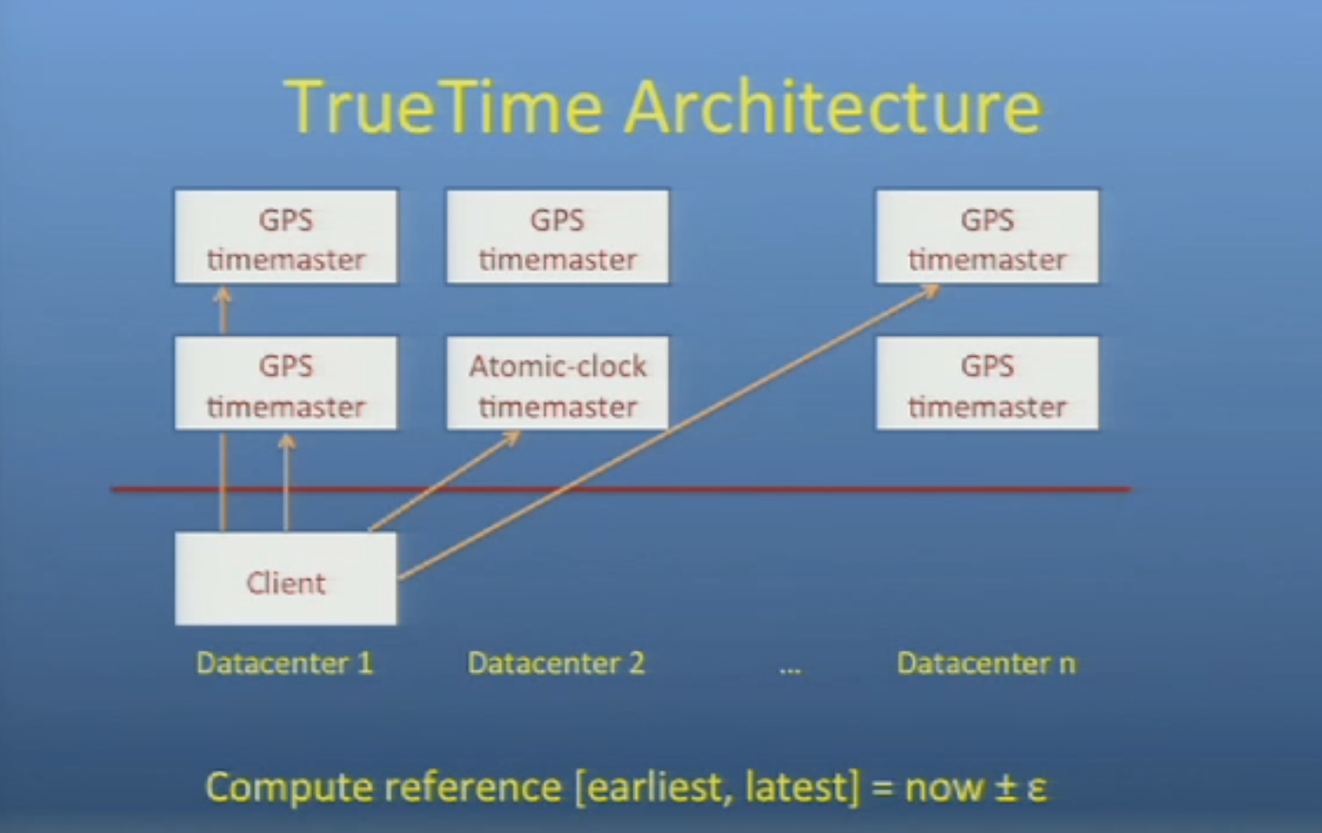
True Time 暴露的接口如下
| Method | Returns |
|---|---|
TT.now() |
TTinterval: [earliest, latest] |
TT.after(t) |
true if t has definitely passed |
TT.before(t) |
true if t has definitely not arrived |
它能保证的是取到的时间误差是有限, 并且可以衡量的(这就有点像ntp了, 但是ntp的误差 比这个大很多, 对于跨全球来说)
6 NTP
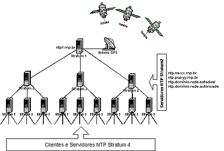
NTP(network time protocol) 最早由D. Mills在1981年提出, 之后成为计算机时间同步的重要协议.
NTP 分为NTP 和 SNTP, 前者基于osi更底层的协议icmp或者ggp(gateway-gateway protocol), 后者基于tcp, 实现思路类似但是具体方法类似(算round trip time), 也有很多个版本, 不同版本间的数据格式可能不太一样. 关于NTP的详细算法描述可以参考, RFC 5905 和 RFC 7822.
NTP server 一般依赖一个外部时钟源(reference clock), GPS and radio time and frequency broadcasts are commonly used as NTP reference clocks.
ntp server 类似于 dns server 都是有一定层级的, 结构大概如下
ntp有几个跟时间同步的精度有关系关键的指标:
-
Stratum: The Stratum of a NTP server denotes its level in the timing hierarchy. A stratum 1 NTP server obtains time from an external timing reference. Stratum 2 devices obtain time from stratum 1 devices and pass timing information to the next level and so on.
-
Jitter: The jitter associated with a timing reference indicates the magnitude of variance, or dispersion, of the signal. Different timing references have different amounts of jitter. The more accurate a timing reference, the lower the jitter value. Jitter is usually measure in milliseconds.
-
Offset: Offset generally refers to the difference in time between an external timing reference and time on a local machine. The greater the offset, the more inaccurate the timing source is. Synchronised NTP servers will generally have a low offset. Offset is generally measured in milliseconds.
-
Delay: Delay in a NTP server describes the round-trip delay or latency of a timing message passed from client to server and back again. The delay is important so that network delays can be calculated and accounted for by a time client.
以上几个指标中, 我们比较关注的是Offset, 就是当前机器的时间和ntp server时间存在的 误差范围, 一般来说都是各位数毫秒, 可以参考如下例子.
当前几乎所有的系统都使用NTP进行时间同步
linux
$ ntpdc -c loopinfo
offset:               -0.000060 s
frequency:            2.822 ppm
poll adjust:          30
watchdog timer:       1942 s
macos
$ sntp -d time.asia.apple.com
sntp 4.2.8p10@1.3728-o Tue Mar 21 14:36:42 UTC 2017 (136~2590)
kod_init_kod_db(): Cannot open KoD db file /var/db/ntp-kod: No such file or directory
handle_lookup(time.asia.apple.com,0x2)
move_fd: estimated max descriptors: 4864, initial socket boundary: 20
sntp sendpkt: Sending packet to 17.253.116.125:123 ...
Packet sent.
sock_cb: time.asia.apple.com 17.253.116.125:123
2019-08-16 11:50:12.990601 (-0800) +0.000296 +/- 0.000380 time.asia.apple.com 17.253.116.125 s1 no-leap
how about windows? 我现在手上没有windows…
以上ntp的对一个客户端显示的offset: -0.000060 s和 +0.000296 +/- 0.000380
就是误差值, 单位秒.
可以看到时间同步的精度还是比较高的.
在David L. Mills的论文中还描述说到, 在21世纪初已经能做到纳秒级别 的时间同步精度. 时间同步的精度应该不是大问题.
7 Logical Clocks and Vector Clocks
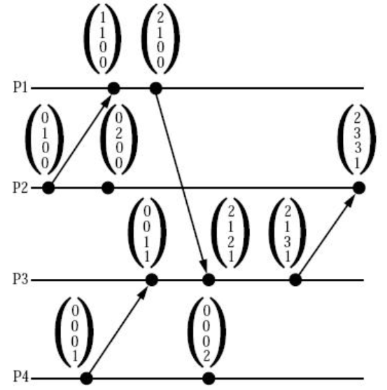
Logical Clocks (Lamport Clocks, LC) and Vector Clocks (Vector Time, VC), 本质上都是 logical clocks, vector clock扩展了logical clocks, 通过使用额外的存储(drawback of vector clocks), 多增加了一个没有Logical clocks没 有的属性.
LC VC 算法概览如下
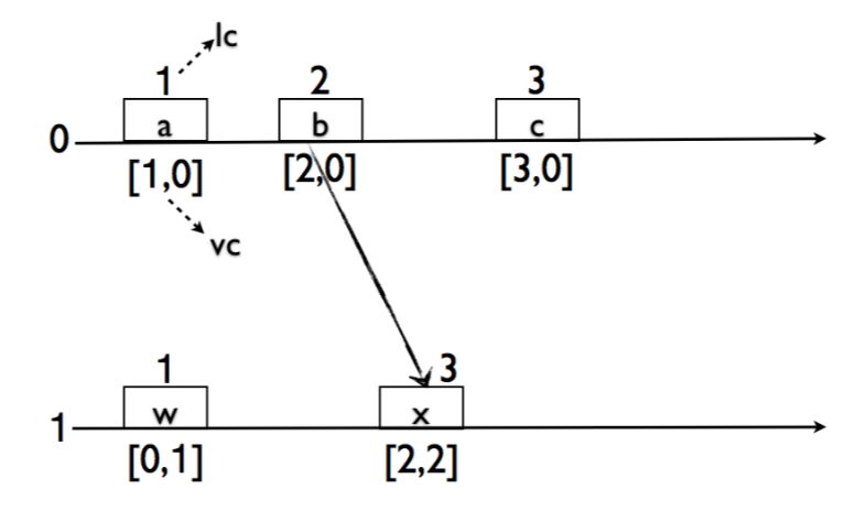
vector clock的大小比较的定义,
For two time vectors
\[u ≤ v \text{ iff } u[i] ≤ v[i] \\ u < v \text{ iff } u ≤ v ∧ u ≠ v, and \\ u || v \text{ iff } \neg (u < v) ∧ \neg(v < u) \\\]基于以上定义, LC, VC 能确保的属性如下
\[e \text{ hb } f ⇒ lc.e < lc.f \\ lc.e = lc.f ⇒ e || f \\ e \text{ hb } f ⇔ vc.e < vc.f \\\]需要注意的是这里边的顺序, 只能保证partial order, 也就是说如果两个节点如果没有交 互则事件的时序是没有办法衡量的, 也就可以认为是并发(\(||\))的.
However, the following claims are not true:
\[e \text{ hb } f ⇐ lc.e < lc.f \\ lc.e = lc.f ⇐ e||f \\ e \text{ hb } f ⇒ pt.e < pt.f \\\]LC/VC有比较明显的缺点:
- 如果集群中有两个节点长时间(永远)没有交互, 那么他们的逻辑时钟计数会相差非常大 (unbounded), 后续提出的HLC很重要的一点就是解决了这个问题.
- 不能体现出事件物理时间上的差距, 如果需要知道比如”3天前”的事件, 逻辑时钟就没法 做到这个
8 Hybrid Logical Clock
HLC 综合了物理时间, 基于NTP不需要额外的硬件, 同时加上了一部分逻辑时钟, 所以称之 为hybrid, HLC算法 克服了LC VC的一些缺点, 使得clock具有物理时间的特性, 同时也能解 决绝大部分分布式系统中的时钟问题, 可以作为一个比较好的True Time替代品.
但是HLC也是有缺点的, 因为基于NTP, 所以它的物理时间误差依赖于NTP, 这个误差主要会影响生成timestamp或者commit wait的性能.
HLC时钟逻辑部分一般是16位, 物理部分一般是43-48位, 物理部分时间单位为毫秒, 一般来 说这个格式也不需要留保留位(高位若干位), 因为一般都是要持久化的, 如果设置了保留位 整个时间戳的处理流程都要为处理保留为留好扩展空间.
HLC时钟选择64位, 据论文里说是为了保持NTP time format一致(方便直接取ntp的高位的若 干位?), 但是我个人认为实际实现 中并没有太大关系, 主要是为了让整个时间简单, 并且 其中物理部分和逻辑部分的位数是可以在具体实现时取合理的值(比如逻辑部分区20位, 物 理部分区44位).
63                                                        15              0
+---------------+-----------------------------------------+---------------+
| reserved(opt) |                 physical                |   logical     |
+---------------+-----------------------------------------+---------------+
                                     l                            c
HLC算法表述如下:
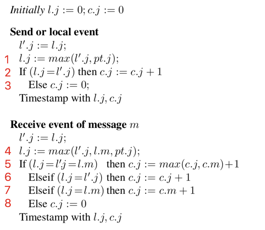
pt: 当前机器的时间, 由ntp进行同步l: hlc时钟的物理部分c: hlc时钟的逻辑部分m: 请求
总结下来:
- 发起请求方的hlc时钟, 按照
pt和l最大值作为hlc的物理部分, 如果hlc物理部分不 变, 则自增c - 请求接收方, 接收到请求之后, 通过比物理时间较来检查是否要更新本地的hlc时钟
- 如果所有的物理时间都一样, 那么接收方的
c就取发起方和接受方的最大c+1 - 如果请求接收方的hlc时钟里的物理时间最大, 则自增接收方的
c - 如果发起方的hlc时钟物理部分大(remote的时间比当前机器时间超前), 则更新本地HLC 时钟, 值为发起方的hlc时钟+1 (物理部分直接赋值, 逻辑部分+1).
- 如果接收方的
pt是所有物理时间里最大, 说明本地机器时间已经向前, 并且本地的l>= 发起方的l,c= 0.
- 如果所有的物理时间都一样, 那么接收方的
显而易见这个算法是保证了在分布式系统中 整个时钟的流向是单调递增的(monotonic).
所有的时间都不会回退, 即使机器上的ntp时间和hlc时钟里的l部分有diff,
这个是非常重要的性质.
以下为HLC的相关性质(hb means happen-before):
Theorem 1. For any two events \(e\) and \(f\),
\[e \text{ hb } f ⇒ (l.e, c.e) < (l.f, c.f)\]Theorem 2. For any event \(f\), \(l.f ≥ pt.f\)
Theorem 3. \(l.f\) denotes the maximum clock value that \(f\) is aware of. In other words,
\[l.f > pt.f ⇒ (∃g : g \text{ hb } f ∧ pt.g = l.f)\]Theorem 4. For any event \(f\),
\[\begin{aligned} c.f = k ∧ k > 0 ⇒ & (\\ & ∃g_1,g_2,··· ,g_k : \\ & (∀j:1≤j<k:g_i\text{ hb }g_i+1) \\ & ∧ (∀j:1≤j≤k:l.(g_i)=l.f) \\ & ∧ g_k \text{ hb } f\\ & ) \\ \end{aligned}\]Corollary 1. For any event \(f\), \(|l.f−pt.f|≤ε\)
Corollary 2. For any event \(f\), \(c.f≤|{g:g\text{ hb }f∧ l.g = l.f)}|\)
Corollary 3. For any event \(f\), \(c.f≤N*(ε+1)\)
Corollary 4. With assumption made below \(c.f ≤ ε/d + 1\). Assumption to reduce the bound on \(c\) further: We assume that the time for message transmission is long enough so that the physical clock of every node is incremented by at least \(d\), where \(d\) is a given parameter.
Theorem 1, 2 and 3 imply the monotonicity of HLC. Corollary 1, 3 and 4 show that \(|l - pt|\) and \(c\) are bounded.
8.1 HLC offset
逻辑部分总共16位, 当所有节点机器物理时间一致时, 单机上同个物理时间点的HLC能提供 65535个timestamp, 物理时间单位是毫秒, 大概每秒能取6千万个timestamp.
对于offset造成性能下降的问题阿里云的博客 是这么描述的
没有偏差的情况下,理论上节点可以做到3千万的TPS,当然在工程上是做不到的。如果两 个节点时钟之间偏移量是5毫秒,那么在5毫秒之内只能通过逻辑时钟去弥补。如果原来6 万个逻辑时钟在1毫秒内就能做完,现在则需要5毫秒,导致整个事务的吞吐下降了600万 。所以时钟偏移会导致peakTPS大幅下降。
如果集群中有两个机器的\(pt\)有明显的差距\(x\), 其实就是说ntp的offset比较大, 根据算法里(7)接收方接收到请求时只能通过递增逻辑部分来弥补, 这样 会导致单个机器上hlc单个物理时 间点上能取到timestamp个数下降, 最差的情况下, 每秒获取timestamp个数下降到(HLC时钟逻辑部分16位):
note: 最差情况下
\[\text{timestamp_per_second} = 65535 × 1000 / (1 + x)\]其中\(x\)为offset的毫秒数, 可以看到, ntp offset越大单位时间内获取timestamp 个数越小
顺便说一下, 个人认为阿里云的博客对应章 节的计算公式是有问题的, 应该要\(+1\), 而不是直接除以\(x\).
下边通过一个例子来说明这种情况.
考虑一个3节点的集群, node1的机器时间超前\(x\)于另外两个节点, 另外两个节点机器时间 一样.
初始条件
\[l_1 = l_2 = l_3 = 0 \\ c_1 = c_2 = c_3 = 0 \\ pt_1 = x \\ pt_2 = pt_3 = 0 \\ pt_1 - pt_2 = x \\ pt_2 - pt_3 = 0 \\\]- node1 给node2 发送了请求, 使用\(l_1 = pt_1 = x\), \(c_1 = 0\)
- node2 接收到请求, 根据HLC算法描述, \(l_2 = l_1 = pt_1 = x\), \(c_2 = 1\), \(pt_2 = 0\) 这个时候\(l_2 - pt = x\)
- node2 给node3 发请求, 使用 \(l_2 = l_1 = pt_1 = x\), \(c_2 = 2\), \(pt_2 = 0\)
- node3 接收到请求, 使用 \(l_3 = l_2 = l_1 = pt_1 = x\), \(c_3 = 3\), \(pt_3 = 0\)
- node2 给node3 发请求, 使用 \(l_2 = l_1 = pt_1 = x\), \(c_2 = 3\), \(pt_2 = 0\)
- node3 接收到请求, 使用 \(l_3 = l_2 = l_1 = pt_1 = x\), \(c_3 = 4\), \(pt_3 = 0\)
- 重复步骤3 4 5 6
可以看到, 如果\(pt_2\)和\(pt_3\)没有达到\(x\)之前的这段时间, 根据HLC算法\(l_2\)和\(l_3\)是没有办法自增的, node2 node3 获取HLC时钟只能自增\(c\)来生成 一个HLC时钟, 也就是说16位的逻辑部分要摊在\(x\)时间来使用, 从而降低了单位时间内获取 timestamp的个数.
当然, 这个是一个非常极端的情况, 如果是node1分别给node2 node3发请求, \(l_2\)和\(l_3\)是 会 随着\(l_1\)的增加而增加的, 而 \(l_1\)是随着\(pt_1\)来增加的, 跟\(pt_2\)和\(pt_3\)就没有关系 了, 这个时候就不存在性能问题.
另外, 值得注意的是, 这里是单机的性能, 如果请求只是从\(pt\)超前的机器上发到其他 机器上, 不会有这个所谓的性能问题.
8.2 Recovery
HLC 中有一条比较重要的性质, 这个按照HLC算法的描述其实是显而易见的.
pt <= l
当若干机器宕机恢复时, 需要确保的是启动的时候 pt 已经大于上一次宕机时的l,
也就是说宕机到恢复期间需要等待一段时间, 否则可能会造成
这批机器间的请求时间”回退”, 这段等待时间长度是可以计算的
论文中, 推论1
|l - pt| <= ε
就是说pt 和 l的最大差值不会超过一个ntp的offset ε, 而一般这个offset最大也就
几百毫秒, 而一个进程从宕机到启动很容易就超过了这个阈值. 如果要确保整个集群已经
持久化下来的timestamp小于启动后的hlc时钟, 那么最好是宕机之后等待一小段时间, 比
如1秒再启动进程.
8.3 Implementation
HLC的实现比较简单, github有一个现成的实现
github.com/cockroachlabs/cockroachdb

cockroach/pkg/util/hlc/hlc.go
基本和自己实现一个类似, 但是抽象了pt的生成, c++中使用system_clock实现pt的
获取应该问题不大. HLC时钟由两部分组成, 如果这两部分使用单独变量存储,
更新的时候需要上锁, 这样实现比较简单, 因为锁中只操作一个变量临界区比较小, 所以还
是可以接受的.
(如果实际实现时发现锁的竞争太激烈导致比较慢, 可以考虑仅使用一个变量来存放HLC时钟,
然后进行原子操作… 应该不需要这么做)
实现时需要考虑几个点:
pt往回跳变需要观察pt和l的diff要控制在maxOffset内, 如果相差太大 系统可能工作就不正常了c部分的溢出检查, 有两种方式:- 直接”进位”到
l上, 但是这么操作可能会违反HLC算法中l - pt <= e的属性, 需 要谨慎操作 - 检测最大值, 如果到达最大值, 当做异常处理
第2种处理方式比较可取, 也有理论验证, 如果有异常了 应该就是ntp时间同步出问题了, 就应该当做异常情况处理.
- 直接”进位”到
8.4 Application
TBD
9 Conclusion
TBD
10 Reference
ntp wikipedia
A Brief History of NTP Time: Confessions of an Internet Timekeeper - David L. Mills
ntp explined
RFC 778
Time, Clocks, and the Ordering of Events in a Distributed System - logical clock
Virtual Time and Global States of Distributed Systems - vector clock
summary of lc, vc, hlc
Synchronization in a Distributed System
Large-scale Incremental Processing Using Distributed Transactions and Notifications
In-depth Analysis on HLC-based Distributed Transaction Processing - alibaba cloud
阿里资深技术专家何登成:基于HLC的分布式事务实现深度剖析
Spanner: Google’s Globally-Distributed Database - Research spanner osdi2012